Toward a Sparse Interpretable Audio Codec
Table of Contents
Introduction
Most widely-used modern audio codecs, such as Ogg Vorbis and MP3, as well as more recent "neural" codecs like Meta's Encodec or Descript's are based on block-coding; audio is divided into overlapping, fixed-size "frames" which are then compressed. While they produce excellent reproduction quality and can be used for downstream tasks such as text-to-audio, they do not produce an intuitive, directly-interpretable representation.
In this work, we introduce a proof-of-concept audio encoder that encodes audio as a sparse set of events and their times-of-occurrence. Rudimentary physics-based assumptions are used to model attack and the physical resonance of both the instrument being played and the room in which a performance occurs, hopefully encouraging a sparse, parsimonious, and easy-to-interpret representation.
We imagine a near-future audio codec where some types of musical composition could take place directly in the audio codec space. Text-to-audio is an excellent interface for non-musicians creating background music for movies, advertisements or social media content, but it is our view that experienced musicians and composers work in a "space" not fully captured by language and will prefer a much finer-grained representation that affords an effectively infinite range of possible sounds.
This work clearly does not replace current music generation models, but could serve as the underlying encoding on which generative models are trained. It is the authors' intuition that models trained on this rich, symbolic representation might have a much deeper "understanding" of the content they produce, given the point-cloud-like nature of the signal. Instead of predicting the next frame, the generative model would be predicting the relationships between "events". Long-term coherence in musical generation has always been a difficult problem, and we speculate that many models spend enormous shares of their capacity learning to reproduce physical resonance, rather than the human forces that drive them in interesting, musical directions.
Early speech results from the LJ-Speech dataset can be found here.
Previous Work
This work takes inspiration from symbolic approaches, such as MIDI, iterative decomposition methods like matching pursuit, and granular synthesis, which represents audio as a sparse set of "grains" or simple audio atoms.
Model
Encoder
The encoder iteratively removes energy from the input spectrogram, producing an event vector and one-hot/dirac impulse
representing the time of occurrence. Other representations of time are possible, e.g., a scalar value of seconds, or
a binary vector representing the frame number with log2(n_samples dimensionality.

Decoder
The decoder uses the 32-dimensional event vector to choose an attack envelope, evolving resonance, and room impulse response to model the acoustic event, and then "schedules" it by convolving the event with the one-hot/direc impulse. Audio is not produced using typical upsampling convolutions, avoiding artifacts and producing more natural-sounding events.
Training Procedure
We train on the MusicNet dataset dataset) for ~76 hours, selecting random ~6 second audio segments sampled at 22050hz (mono) with a batch-size of 2. The model takes the following steps for 32 iterations on each training sample:
- The encoder analyzes the STFT spectrogram of the signal, producing a single 32-dimensional event vector and a one-hot vector representing time-of-occurrence
- The decoder produces "raw" audio samples of the acoustic event
- an STFT spectrogram of the acoustic event is produced and subtracted from the input spectrogram
- The encoder analyzes the residual and the process is repeated
The model is trained to maximize the amount of energy removed from the original signal at each step, and to minimize an adversarial loss, produced by a small, convolutional down-sampling discriminator which is trained in parallel, analyzing both the real and reproduced signals in the STFT spectrogram domain. Half of the generated events are masked/removed when analyzed by the discriminator, encouraging each event vector to stand on its own as a realistic event.
All training and model code can be found here.
Streaming Algorithm
When encoding, the entire ~6-second spectrogram is analyzed, but its second-half is masked when choosing the next event. In this way, the model can slide along overlapping sections of audio and encode segments of arbitrary durations.
Future Work
Better Perceptual Audio Losses
Recent experiments use a greedy, per-event loss which maximizes the energy removed from the signal at each step, as well as a learned, adversarial loss. Reconstruction quality will likely benefit from a more perceptually-aligned loss and a larger, more diverse dataset.
Model Size, Training Time and Dataset
Firstly, this model is relatively small, weighing in at ~14M parameters (~80 MB on disk) and has only been trained for around 76 hours, so it seems there is a lot of space to increase the model size, dataset size and training time to further improve. The reconstruction quality of the examples on this page is not amazing, certainly not good enough even for a lossy audio codec, but the structure the model extracts seems like it could be used for many interesting applications, and future work will improve perceptual audio quality.
Different Event Generator Variants
The decoder side of the model is very interesting, and all sorts of physical modelling-like approaches could yield better, more realistic, and sparser renderings of the audio.
For example, simple RNNs might serve as a natural alternative to the encoder used for the sound reproductions in this article.
Cite this Article
If you'd like to cite this article, you can use the following BibTeX block.
Streaming Algorithm for Arbitrary-Length Audio Segments
In this latest iteration of the work, we introduce a "streaming" algorithm so that we can decompose audio segments of arbitrary lengths.
Original (Streaming)
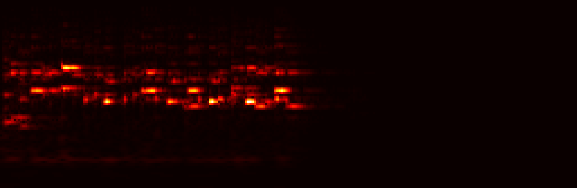
Reconstruction (Streaming)
Audio Examples
Example 1
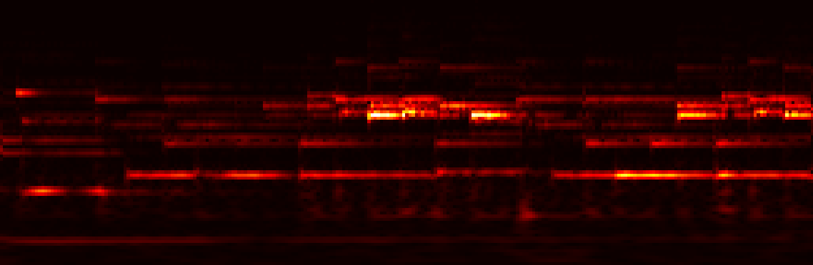
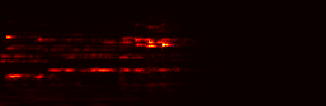
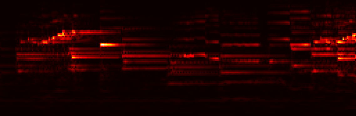
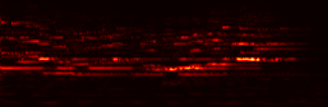
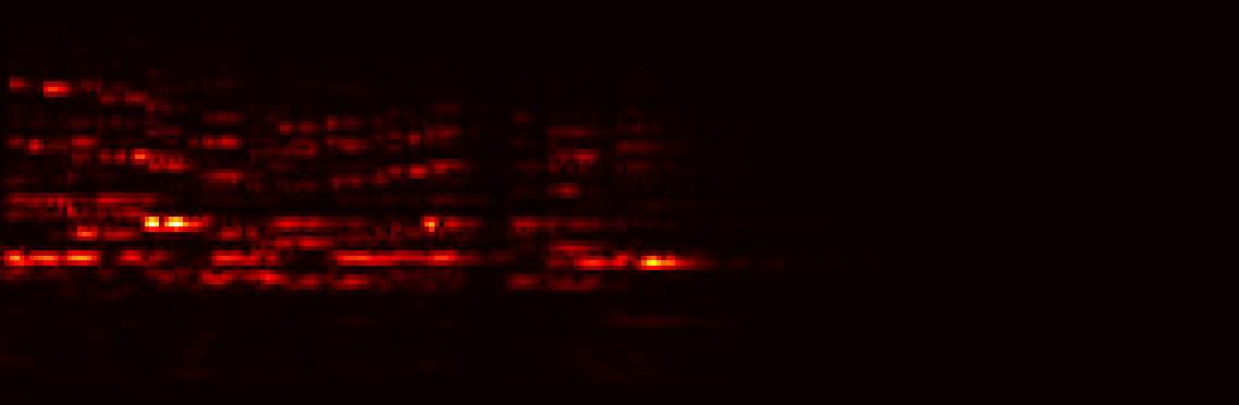
Original Audio
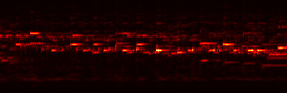
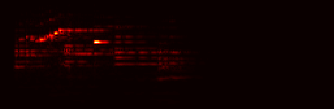
Reconstruction
We mask the second half of the input audio to enable the streaming algorithm, so only the first half of the input audio is reproduced.
Event Scatterplot
Time is along the x-axis, and a 32D -> 1D projection of event vectors using t-SNE constitutes the distribution along the y-axis.
Colors are produced via a random projection from 32D -> 3D (RGB). Here it becomes clear that there are
many redundant/overlapping events. Future work will stress more sparsity and less event overlap,
hopefully increasing interpretability further.
Individual Event Intermediate Steps
Here, we choose an individual event at random and demonstrate the intermediate decoder steps, including the original energy "impulse", the choice of resonance, and finally, the choice of a room impulse response.
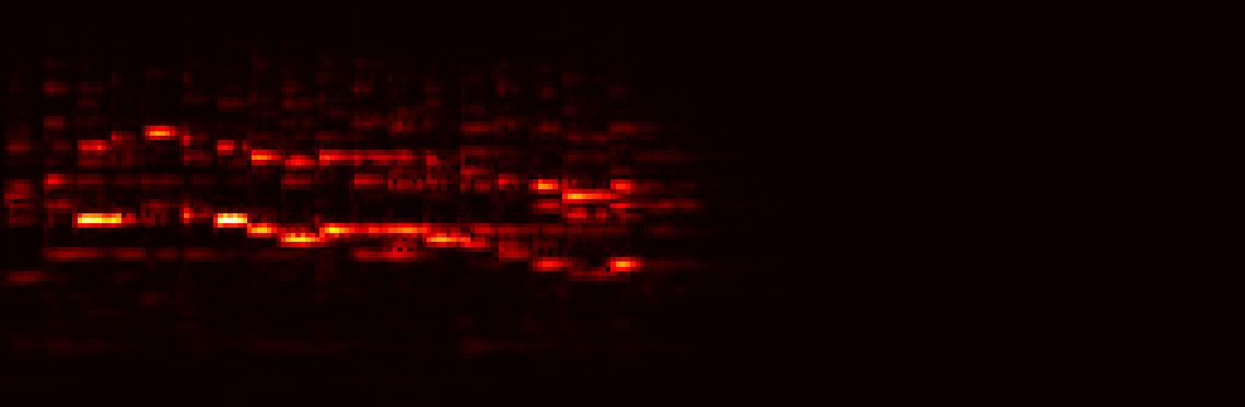
Energy Impulse

Energy Convolved with Chosen Resonances

Deformation/Interpolation Between Chosen Resonances Over Time

Signal Convolved with Room Impulse Response

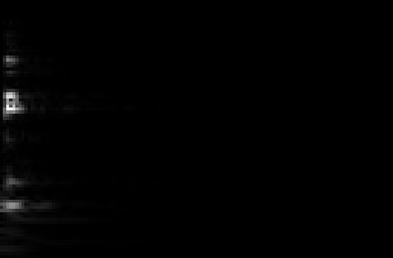
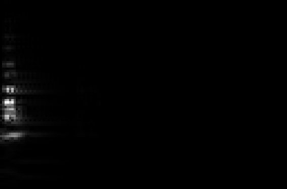
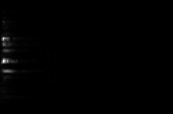
Decomposition Process
We can see that while energy is removed at each step, removed segments do not map cleanly onto audio "events" as a human listener would typically conceive of them. Future work will move toward fewer and more meaningul events via induced sparsity and/or clustering of events.
Randomized
Here, we generate random event vectors with the original event times.
Here we use the original event vectors, but choose random times.
Random Perturbations
Each event vector is "perturbed" or moved in the same direction in event space by adding a random event vector with small magnitude
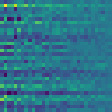
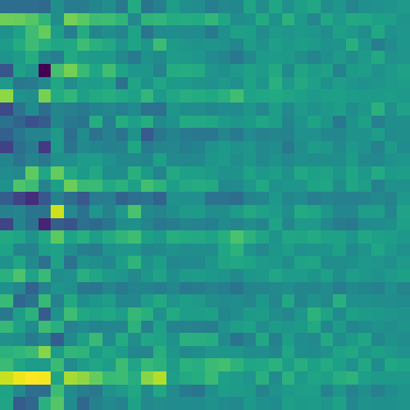
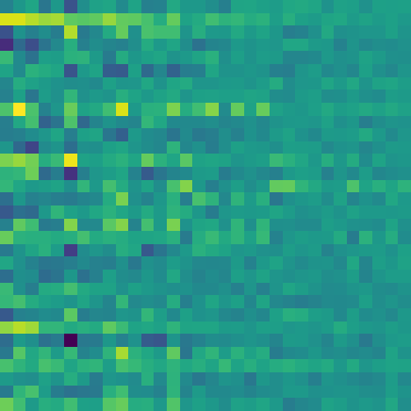
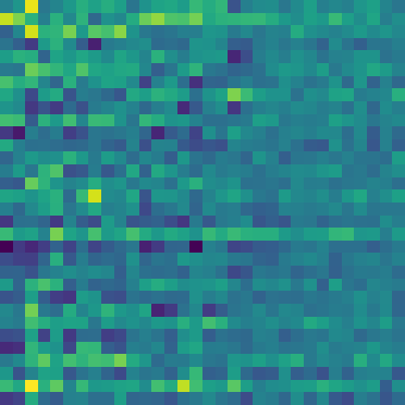
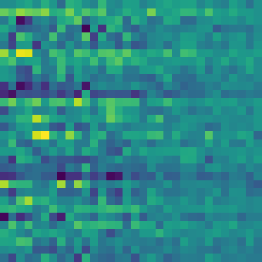
Event Vectors
Different stopping conditions might be chosen during inference (e.g. norm of the residual) but during training, we remove energy for 32 steps.
Each event vector is of dimension 32. The decoder generates an event from this vector, which is then scheduled.
Example 2
Original Audio
Reconstruction
We mask the second half of the input audio to enable the streaming algorithm, so only the first half of the input audio is reproduced.
Event Scatterplot
Time is along the x-axis, and a 32D -> 1D projection of event vectors using t-SNE constitutes the distribution along the y-axis.
Colors are produced via a random projection from 32D -> 3D (RGB). Here it becomes clear that there are
many redundant/overlapping events. Future work will stress more sparsity and less event overlap,
hopefully increasing interpretability further.
Individual Event Intermediate Steps
Here, we choose an individual event at random and demonstrate the intermediate decoder steps, including the original energy "impulse", the choice of resonance, and finally, the choice of a room impulse response.
Energy Impulse

Energy Convolved with Chosen Resonances

Deformation/Interpolation Between Chosen Resonances Over Time

Signal Convolved with Room Impulse Response
Decomposition Process
We can see that while energy is removed at each step, removed segments do not map cleanly onto audio "events" as a human listener would typically conceive of them. Future work will move toward fewer and more meaningul events via induced sparsity and/or clustering of events.
Randomized
Here, we generate random event vectors with the original event times.
Here we use the original event vectors, but choose random times.
Random Perturbations
Each event vector is "perturbed" or moved in the same direction in event space by adding a random event vector with small magnitude
Event Vectors
Different stopping conditions might be chosen during inference (e.g. norm of the residual) but during training, we remove energy for 32 steps.
Each event vector is of dimension 32. The decoder generates an event from this vector, which is then scheduled.
Example 3
Original Audio
Reconstruction
We mask the second half of the input audio to enable the streaming algorithm, so only the first half of the input audio is reproduced.
Event Scatterplot
Time is along the x-axis, and a 32D -> 1D projection of event vectors using t-SNE constitutes the distribution along the y-axis.
Colors are produced via a random projection from 32D -> 3D (RGB). Here it becomes clear that there are
many redundant/overlapping events. Future work will stress more sparsity and less event overlap,
hopefully increasing interpretability further.
Individual Event Intermediate Steps
Here, we choose an individual event at random and demonstrate the intermediate decoder steps, including the original energy "impulse", the choice of resonance, and finally, the choice of a room impulse response.
Energy Impulse

Energy Convolved with Chosen Resonances
Deformation/Interpolation Between Chosen Resonances Over Time

Signal Convolved with Room Impulse Response

Decomposition Process
We can see that while energy is removed at each step, removed segments do not map cleanly onto audio "events" as a human listener would typically conceive of them. Future work will move toward fewer and more meaningul events via induced sparsity and/or clustering of events.

Randomized
Here, we generate random event vectors with the original event times.
Here we use the original event vectors, but choose random times.
Random Perturbations
Each event vector is "perturbed" or moved in the same direction in event space by adding a random event vector with small magnitude
Event Vectors
Different stopping conditions might be chosen during inference (e.g. norm of the residual) but during training, we remove energy for 32 steps.
Each event vector is of dimension 32. The decoder generates an event from this vector, which is then scheduled.
Example 4
Original Audio
Reconstruction
We mask the second half of the input audio to enable the streaming algorithm, so only the first half of the input audio is reproduced.
Event Scatterplot
Time is along the x-axis, and a 32D -> 1D projection of event vectors using t-SNE constitutes the distribution along the y-axis.
Colors are produced via a random projection from 32D -> 3D (RGB). Here it becomes clear that there are
many redundant/overlapping events. Future work will stress more sparsity and less event overlap,
hopefully increasing interpretability further.
Individual Event Intermediate Steps
Here, we choose an individual event at random and demonstrate the intermediate decoder steps, including the original energy "impulse", the choice of resonance, and finally, the choice of a room impulse response.
Energy Impulse

Energy Convolved with Chosen Resonances

Deformation/Interpolation Between Chosen Resonances Over Time

Signal Convolved with Room Impulse Response

Decomposition Process
We can see that while energy is removed at each step, removed segments do not map cleanly onto audio "events" as a human listener would typically conceive of them. Future work will move toward fewer and more meaningul events via induced sparsity and/or clustering of events.
Randomized
Here, we generate random event vectors with the original event times.
Here we use the original event vectors, but choose random times.
Random Perturbations
Each event vector is "perturbed" or moved in the same direction in event space by adding a random event vector with small magnitude
Event Vectors
Different stopping conditions might be chosen during inference (e.g. norm of the residual) but during training, we remove energy for 32 steps.
Each event vector is of dimension 32. The decoder generates an event from this vector, which is then scheduled.
Example 5
Original Audio

Reconstruction
We mask the second half of the input audio to enable the streaming algorithm, so only the first half of the input audio is reproduced.
Event Scatterplot
Time is along the x-axis, and a 32D -> 1D projection of event vectors using t-SNE constitutes the distribution along the y-axis.
Colors are produced via a random projection from 32D -> 3D (RGB). Here it becomes clear that there are
many redundant/overlapping events. Future work will stress more sparsity and less event overlap,
hopefully increasing interpretability further.
Individual Event Intermediate Steps
Here, we choose an individual event at random and demonstrate the intermediate decoder steps, including the original energy "impulse", the choice of resonance, and finally, the choice of a room impulse response.
Energy Impulse

Energy Convolved with Chosen Resonances

Deformation/Interpolation Between Chosen Resonances Over Time

Signal Convolved with Room Impulse Response
Decomposition Process
We can see that while energy is removed at each step, removed segments do not map cleanly onto audio "events" as a human listener would typically conceive of them. Future work will move toward fewer and more meaningul events via induced sparsity and/or clustering of events.
Randomized
Here, we generate random event vectors with the original event times.
Here we use the original event vectors, but choose random times.
Random Perturbations
Each event vector is "perturbed" or moved in the same direction in event space by adding a random event vector with small magnitude
Event Vectors
Different stopping conditions might be chosen during inference (e.g. norm of the residual) but during training, we remove energy for 32 steps.
Each event vector is of dimension 32. The decoder generates an event from this vector, which is then scheduled.
Notes
This blog post is generated from a Python script using conjure.